Refine Relock Outline

I. Build Relevant Span -- get_relevant_span(name, vs)

a) Takes in a time from /data/users/class/mapmaking_in/dtod/{band}/{file}$ ls in terminal and finds predicted relocks during the given time stamp.

b) Returns the span for the data that closely surrounds (20 minutes before and 20 minutes after) the first predicted relock in the list of relock locations. Also returns the ctime of the predicted relock (tod_relocs_old) and the index of the predicted relock (ctime_inds).

II. Make Groups -- make_groups(span, vs)

• For the w1_6 band, I have found that the detectors are split into 4 groups based on when their relocks occur (for example, detectors 0 through 160 all have relocks occur at the same time; Detectors 180 through 247 always have their relocks occur at the same time; etc.). I will call these groups relock groups.

• However, the boundaries of these 4 groups of detectors isn't the same for every timespan, so I determined which detectors were generally on the boundary between relock groups. I did this by plotting the data for all detectors for several different timespans. I then manually inspected where the boundary between relock groups were (by observing when the relock location shifted). I then added the two detectors before and two detectors after the shift to their corresponding list of intermediate detectors. There is one list of intermediate detectors for each boundary between relock groups -- so there are 3 intermediate groups in total. I found that the intermediate groups are as follows:

  • intermediate group 1 (i_group_1_orig): 162, 164, 167, 169, 176, 179 -- between relock groups 1 and 2
  • intermediate group 2 (i_group_2_orig): 249, 258, 262, 263, 265, 270 -- between relock groups 2 and 3
  • intermediate group 3 (i_group_3_orig): 425, 426, 433, 434, 440, 449 -- between relock groups 3 and 4

• I found that occassionally the detectors that are present aren't the same for all spans. Due to this, I built the relock groups based on the intermediate detectors that do exist for the given span. For example, if detector 162 is present for a given span, then group 1 encompasses all detectors from the first detector to the detector preceding 162. If detector 162 is not present, then group 1 encompasses the first detector to the detector preceding 164.

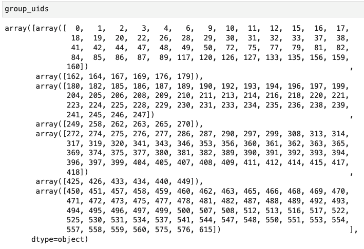
• Note: This function returns group_1, i_group_1, group_2, ... which are lists containing the data for the detectors in their respective groups. I don't think I ended up using these variables in the rest of this method. Instead, I found it easier to use group_uids, which is also returned by this function. group_uids is an array of 7 arrays, each containing the detectors in a given group -- ordered: group 1, i group 1, group 2, i group 2, group 3, i group 3, group 4

• Example of group_uids before the intermediate detectors are assigned:

III. Refine Relock Location for Each Relock Group -- refine_reloc_locs_w1_6(span, initial_loc, win)

• This uses the original moby2 refine relock operation on each relock group. However, since I couldn't directly implement the moby2 refine relock, I basically rewrote the operation to work within the system I am using right now.

• Part of implementing the original operation is finding the paired and unpaired detectors then making an array of the positive and negative paired detectors. Obtaining these results is already programmed into moby2 and Dpipe, however I couldn't find a way to do this for only a select group of detectors. Because of this, I added wrote two functions to do this process -- get_paired_unpaired(span) and get_plus_minus_dets(all_paired_dets, group)

• Once you have the information provided by these functions, we can use the original refine relock operation on the 4 groups with the intermediate detectors excluded. On several occassions, two or more of the refined locations would be sequential and the rest would be far off of the correct location. Via inspection, I concluded that the relock locations should be in sequential order by index, which makes sense considering the groups are likely in sequential samples. Because of this, I wrote another function, find_seq_locs(relock_locations) to take the output of the list of moby2 style refined relock locations (indices), find which locations/indices are sequential, and adjust the other relock indices to fit within that sequential order

  • Note: I am not completely sure that it is safe to assume that the relocks are in sequential indices, however, I haven't had an issue with this assumption so far.

IV. Assign Intermediate Detectors to Relock Groups -- assign_group(span, det, group, relock_locs, bound, failed_already)

• This method is fairly complicated and is likely most easily understood with a flow chart; so I have made one and attached it below.
• As you can see, there are 4 methods I used to determine which group a given detector belongs to. The goal of these methods is to find where relocks occur individually for a detector. I will go through those methods here.
• The type of relock is also tracked throughout the function as booleans (a separate one for each type) and returned at the end.

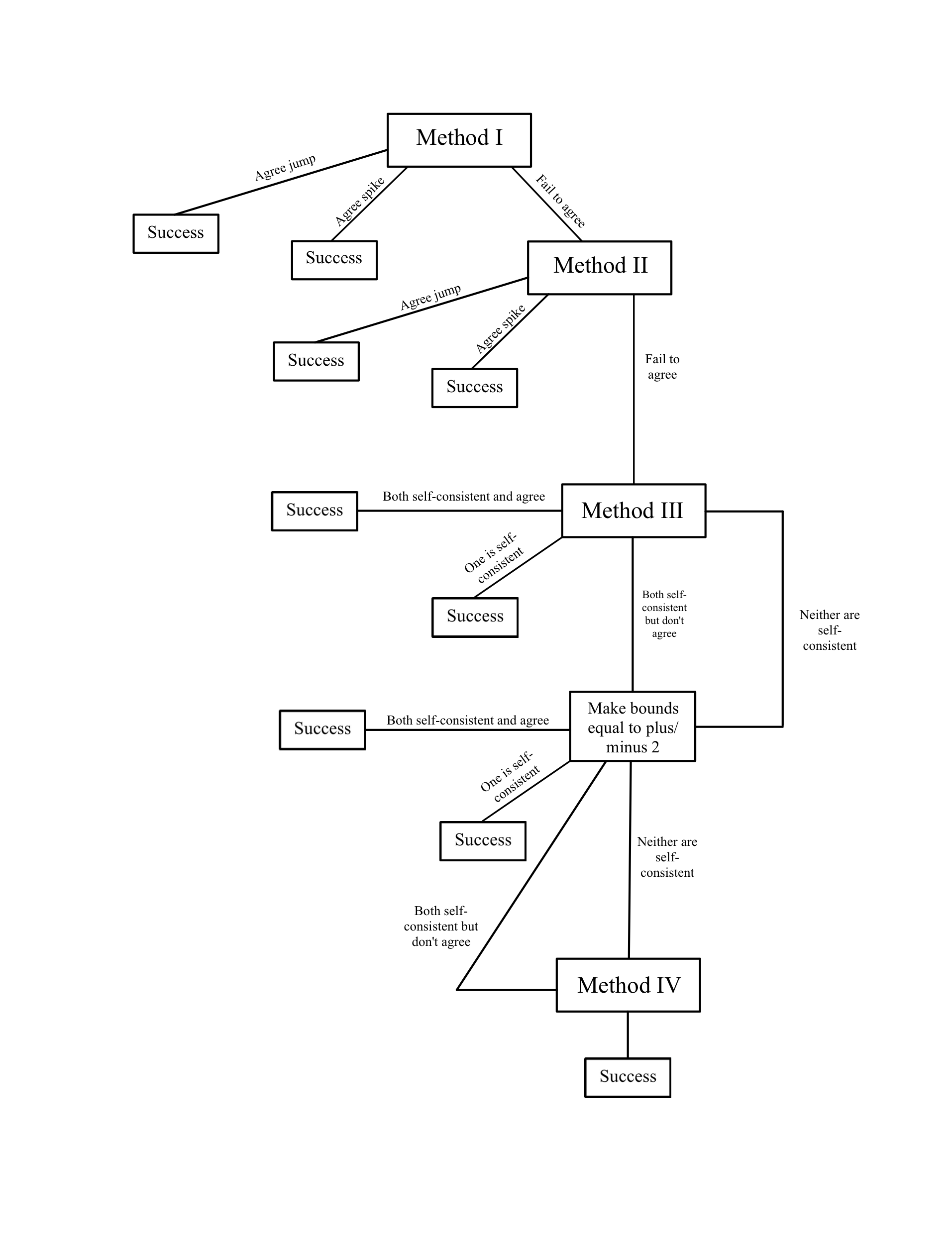
Method I:

• This is the first method that is tried and it occurs directly in the assign_group() method, so there is no separate function defining this operation.

• This method revolves around determining whether the relock is a jump or a spike, which will allow us to mathematically determine the relock location.

• For a given relock location (either the one preceding or succeeding the intermediate group this detector is in), I find the difference between the data 3 indices before the relock (lower_bound) and 3 indices after the relock (upper_bound). If the absolute value of that difference is greater than a certain parameter, then the relock is a jump. If the difference is less than the parameter, then the relock is a spike. The parameter is set at the difference between min and max of all data between the upper and lower bounds, divided by 2.

• To check for consistency, I do this method with both relock locations preceeding and succeeding the intermediate group the detector is in.

   

• If the method concludes that the relock is a jump regardless of which relock location used, then the relock location is found by:

  • a) Take the data 5 indices before the lower bound and 5 indices after the upper bound. Append these into one array, defined as surrounding_data
  • b) Take the average of the data in surrounding_data, saved as average
  • c) Iterate through all relock indices (relock_locs) and take the difference between the average and the data at the relock location -- append this value to a differences array. The difference should decrease as the relock locations get closer to the actual relock location, and increase once it has passed it.
  • d) I track whether or not the index is already past the average -- I am not completely sure if this is necessary.
  • e) The index of the minimum of the differences array tells us which group the relock index is closest to.
  • f) Finally, I assign the detector to the adjacent group (aka one of the two groups that the intermediate group is between) that is closest to the group determined in the previous part
    • I added this part in because there were times where the method returned that the relock location was closest aligned to a non-adjacent relock group.
    • This is done by making an array of the differences between the adjacent group numbers and the number of the group closest to the mathematically isolated relock location.
  • Example:

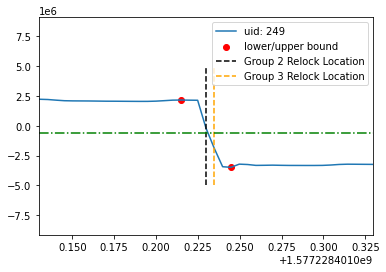
• The upper and lower bounds in the graph represent the bounds for the latter relock group

 

• If the method concludes that the relock is a spike regardless of which relock location is used, then the relock location is found by:
  • a) Similar to the approach for jumps, this operation starts off by defining the surrounding data and finding the average of it.
  • b) After this, the data is normalized by subtracting all values between the lower and upper bound by the average.
  • c) Next, I take the absolute value of every data point of the normalized data (I take the absolute value to avoid needing to worry about negatives in the next step).
  • d) Naturally, the index where the max of the absolute value data occurs is the index of the relock (plus the index of the lower bound... Can't forget that the absolute value data actually starts at the index saved as lower_bound)
  • e) I iterate through the relock indices and append their difference from the relock index (set in the previous part) to a difference array.
  • f) Like with the jumps, the index of the minimum difference tells us which group the relock is closest to.
  • g) Again, similar to the jumps, I then find which adjacent group is closest to the group that was returned in the previous part. This is done in the same was as it is for the jumps
  • Example:

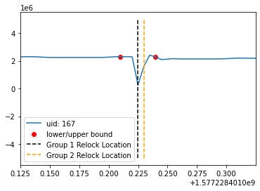
• The upper and lower bounds in the graph represent the bounds for the latter relock group

 

• If the method fails to produce agreement amongst locations on whether the relock is a spike or jump, then fail == True. In this case, Method II (method_0()) is called.

Method II (method_0):

• This method function quite similarly Method I (Method I is NOT the same as method_1 -- I apologize for the confusing naming conventions), with the only difference being the choice of bounds.

   

• For this method, two new choices of bounds are tried:
  • 1. Lower Bound = lower bound from lower relock group; Upper Bound = upper bound from higher relock group
  • 2. Lower Bound = lower bound from higher relock group; Upper Bound = upper bound for lower relock group

        

• This effectively creates two new bounds -- one wider and the other narrower.
• Like in the previous method, we test for agreement on the type of relock. The operation that is used if there is agreement (on spike or jump) is the same as the previous method.
• If it fails to produce agreement, then we move on to Method III (method_1).

Method III (method_1):

• This method is very similar to the last method in that it is essentially the same as the original method except that the bounds are different.

• In this method, we test another pair of bounds to see if we can get any agreement. In this case, one set of bounds is 1 indices narrower than the original and the other is 1 indices wider than the original. This is done by calling assign_group() with the new bounds.

  • In order to prevent this method from calling the method it exists within and potentially causing an endless loop, I added a boolean variable, failed_already, and made it a part of the implementation of the assign_group(). I then included the condition that failed_already != True for it to enter method_0. failed_already is always set to False upon intialization.

     

• If calling assign_group() with the two new sets of bounds produces self-consistent results AND the results amongst the two bounds are the same, then we can take this as the result we are looking for.

• If calling assign_group() with one of new bounds (either narrower or wider) doesn't fail (aka, it produces agreement internally) but the other does, then we can use the solutions of the group that works.

• If both bounds produces self-consistent results, but don't agree with each other (rarely happens), then we increase the bounds further. We now call assign_group() with two more sets of bounds -- one that is 2 indices narrower than the original and another that is 2 indices wider than the original.

  • In this case, we proceed just like we did with the first set of new bounds in this new method:
  • if they are both self-consistent (fail == False) and they produce agreement between them on results, then we can accept the answers they produce.
  • if one produces agreement but the other fails, then we can take the results of the one that succeeds.
  • if the both fail, then we can go to Method IV (method_2)
  • if they succeed (aka are self-consistent), but don't agree with each other, then we move on to Method IV (method_2)

     

• If both set of bounds fail, we do the same process as the previous bullet point.

• then we can take the results as the final results, as long as there is agreement. For example, if the wider bounds fails to produce agreement internally (assign_group() returns fail = True) but the narrower bounds produce a consistent answer, then we can take the result from the narrower bounds; and vice versa.

• However, if both new bounds succeed in producing self-consistent results but the results aren't consistent with each other, then this method fails.

• If neither of the new bounds succeed in producing

Method IV (method_2):

• If the algorithm has made it this far, then the relock likely neither a jump nor a spike. When it is not a jump or a spike, the relock is generally somewhat "chaotic" then relatively flat after the relock occurs from what I have seen.

• This last method finds the location for this case.

• In theory, whichever relock location shows greater variability on one side of it than on the other is the location that is closest to the actual relock location (the point where things change). Here's how I encoded this process:

• For each adjacent relock location:

  • The algorithm takes data from the left of the relock location and finds the absolute value of the difference between max and min on the left. We will call this value the variability. Do this for the right as well.
  • Subtract the variability of the left from the variability of the right and take the absolute value. We will call this variable difference in the code.

• Finally, whichever group produces the greatest variability is the group that the detector belongs to. Also, return choas_to_flat = True, because this is how I chose to denote this type of detector.

• (Another method could be to compare the variance of right to left for each relock location, then compare the relock locations against each other)

• In the end, assign_group() returns the number of the group the detector belongs to (numbered starting with 0), and boolean values for jump, spike, fail, and choas_to_flat, which reveals what type of relock it is. Returning fail = True is only relevant within the method itself. The method will never return fail = True as the final result

V. Remake Groups -- remake_groups(span, group_uids, relock_locs)

• Iterate through all intermediate detectors and call assign_group for each.
• Append the uids of the detectors to the their corresponding relock group (which is the result of assign_group). Remember that assign_group returns the group number starting at 0
  • Starting at 0 is advantageous because we can easily find the index that the detector uid should be appended to in the group_uids array (which has the uids for all 7 groups -- main and intermediate) by multiplying the result of assign_groups by 2.
• Finally, the intermediate groups are deleted at the end after all of the detectors in all intermediate groups have been assigned to main groups.
• The new detector groups are returned.

VI. Final Product -- do_relock_calcs(span, ctime_inds)

• This basically does all of the key functions that were just mentioned, at once.
• It takes a span and the index of the predicted/scheduled relocks as inputs
• Makes the groups with make_groups()
• Calculates the relock locations with refine_reloc_loc_w1_6()
• Remakes the groups, assigning the intermediate detectors to groups using remake_groups()
• It sorts the detector uids within the groups in the new array of group uids
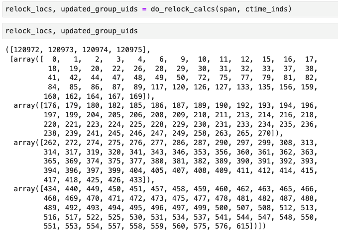
• Finally, it returns the location of the relocks for the 4 groups and an array of arrays with axis=0 being the groups and axis=1 being the detectors in the respective groups.
• Example output: